Summary

In this activity I explore the relationship between team performance and team pressure behavior using data from the English Premiere League season 2020-2021. I focus on Manchester City and Sheffield United, respectively the winner and bottom finisher for that season. I describe how points, goals-against (GA) and shots-on-target-against (SoTA) are related to the success rate and the field location of teams’ pressure acvitivies, and how these relationships explai the different final placements achieved by high-perfoming and low-performing teams. The analyzed metrics are related to passes-per-defensive action (PPDA), a summary metric of a team’s efficiency in applying defensive pressure, but in this note I do not look at this metric. Instead I focus on readily available, first-principles metrics that are nonetheless informative with only a minimum of data processing. While my observations are qualitative, they are supported by quantitative and exploratory analyses performed in Python.

While high-press (applying defensive pressure in the opponent’s third of the pitch) is not required for teams to win games, there exist a correlation between winning (points achieved) and using high-press. However, it is not sufficient to simply apply pressure (proximity within 5 meters of an opponent with the ball) in quantity in the attacking third: the quality of the pressure is also important, as measured by the success rate of pressure events (success is winning possession). Furthermore, it is important to also look at the normalized profiles of pressure events across the thirds of the pitch to characterize how a team chooses to distribute its totall pressure effort throughout a match in the three zones: raw counts, even segmented by pitch thirds, are misleading.

For the purposes of analysing a team’s pressure effectiveness, metrics closer to the played game such as GA and SoTA are more relevant than points earned. For these metrics there is a stronger correlation with the success rate of pressure and the proportion of pressure applied in the attacking third.

The statistics of Sheffield United (bottom-finisher) and Manchester City (EPL winner), are surprising at first if we only consider points won. Sheffield produced the highest number of pressures, both in total and in the attacking third, but finished last. Manchester City, conversely, had the fewest number of pressures, yet was the winner. The distinguishing characteristic for Man City is the highest success rate of the pressures and its stronger propensity toward the high-press.

Success in pressure depends on many factors. It is not limited to the individual pressure event that leads to winning possession, but it also depends on the teammates covering the spaces or marking 1:1 correctly, applying their chosen pressure structures correctly, being ready on their jumps-to-pressure, and on any dynamic advantage of the individual players. Manchester City possesses more of these team and individual characteristics than Sheffield United and it is likely better able to choose the moments for applying pressure, increasing the efficiency of pressure activities. This, together with the fact that they practice a higher press, contributes to their low GA and SoTA metrics.

Data

The data was downloaded from FBRef. This exercise is part of the requirements for the course “High-press in Football” from Barca Innovation Hub

Set up the Python environment, load and prepare data

Code

import pandas as pd
from google.colab import data_table
import seaborn as sns
sns.set_theme('talk')
import matplotlib.pyplot as plt

Code

# Read the Squads and Players --> defensive actions statistics
data_source = 'https://fbref.com/en/comps/9/10728/defense/2020-2021-Premier-League-Stats#stats_squads_defense_for'
pressure_data = pd.read_html(data_source)[0]

#Keep only what we need
pressure_data = pressure_data[['Unnamed: 0_level_0', 'Pressures']].copy()
pressure_data.columns  = pressure_data.columns.droplevel()

# Calculate the percentage of pressure events by third of the field --> will use it later
# Rounding the numbers for readability
pressure_data['Def 3rd %'] = round(pressure_data['Def 3rd']/pressure_data['Press'] * 100,1)
pressure_data['Mid 3rd %'] = round(pressure_data['Mid 3rd']/pressure_data['Press'] * 100, 1)
pressure_data['Att 3rd %'] = round(pressure_data['Att 3rd']/pressure_data['Press'] * 100, 1)

# Read the Squads and Players --> goalkeepeing statistics
goalkeeping_source='https://fbref.com/en/comps/9/10728/keepers/2020-2021-Premier-League-Stats#stats_squads_keeper_for'
goalkeeping_data = pd.read_html(goalkeeping_source)[0]

#Keep only what we need
goalkeeping_data.drop(['Penalty Kicks', 'Playing Time', 'Unnamed: 1_level_0'], axis=1, inplace=True, level=0)
goalkeeping_data.columns = goalkeeping_data.columns.droplevel()

# Calculate the total points for the season for each team --> will use it later 
goalkeeping_data['Points'] = 3*goalkeeping_data['W'] + goalkeeping_data['D']

# Keep only what we need
goalkeeping_data.drop(['Saves', 'Save%', 'W', 'D', 'L', 'CS', 'CS%'], axis=1, inplace=True)

Code

# Finally, let's inspect the table
all_data = pd.merge(pressure_data, goalkeeping_data, on='Squad')
data_table.DataTable(all_data, include_index=False)

	Squad	Press	Succ	%	Def 3rd	Mid 3rd	Att 3rd	Def 3rd %	Mid 3rd %	Att 3rd %	GA	GA90	SoTA	Points
0	Arsenal	4685	1331	28.4	1499	1897	1289	32.0	40.5	27.5	39	1.03	128	61
1	Aston Villa	5446	1473	27.0	1888	2277	1281	34.7	41.8	23.5	46	1.21	177	55
2	Brighton	5179	1638	31.6	1732	2164	1283	33.4	41.8	24.8	46	1.21	117	41
3	Burnley	4654	1282	27.5	1381	2041	1232	29.7	43.9	26.5	55	1.45	179	39
4	Chelsea	5376	1668	31.0	1692	2388	1296	31.5	44.4	24.1	36	0.95	103	67
5	Crystal Palace	5700	1502	26.4	2314	2378	1008	40.6	41.7	17.7	66	1.74	173	44
6	Everton	5660	1604	28.3	2220	2364	1076	39.2	41.8	19.0	48	1.26	158	59
7	Fulham	5145	1537	29.9	1720	2157	1268	33.4	41.9	24.6	53	1.39	164	28
8	Leeds United	6661	1972	29.6	2341	2885	1435	35.1	43.3	21.5	54	1.42	189	59
9	Leicester City	5142	1629	31.7	1797	2214	1131	34.9	43.1	22.0	50	1.32	134	66
10	Liverpool	5394	1707	31.6	1339	2329	1726	24.8	43.2	32.0	42	1.11	137	69
11	Manchester City	4560	1462	32.1	1167	2030	1363	25.6	44.5	29.9	32	0.84	89	86
12	Manchester Utd	5041	1490	29.6	1537	2164	1340	30.5	42.9	26.6	44	1.16	135	74
13	Newcastle Utd	5423	1346	24.8	2148	2247	1028	39.6	41.4	19.0	62	1.63	179	45
14	Sheffield Utd	6123	1518	24.8	2080	2631	1412	34.0	43.0	23.1	63	1.66	205	23
15	Southampton	5714	1783	31.2	1970	2500	1244	34.5	43.8	21.8	68	1.79	169	43
16	Tottenham	5871	1643	28.0	2124	2563	1184	36.2	43.7	20.2	45	1.18	144	62
17	West Brom	5491	1531	27.9	2119	2268	1104	38.6	41.3	20.1	76	2.00	235	26
18	West Ham	4989	1342	26.9	1882	2133	974	37.7	42.8	19.5	47	1.24	143	65
19	Wolves	5195	1558	30.0	2105	2187	903	40.5	42.1	17.4	52	1.37	144	45

Code

# Define some functions to help the visualizations
def plot_squads(df, x, y, figsize=(10,10), fontdict=dict(size=10),
                title='', xlabel='', ylabel='', x_offset=0.1, y_offset=0.1):
  plt.figure(figsize=figsize)
  sns.scatterplot(data=df, x=x, y=y)
  plt.title(title)
  plt.ylabel(ylabel)
  plt.xlabel(xlabel)
  for _, row in df.iterrows():
    plt.text(row[x]+x_offset, row[y]+y_offset, row['Squad'], fontdict=fontdict)


def subplot_squads(df, x, y, ax, fontdict=dict(size=10),
                   xlabel='', ylabel='', x_offset=0.1, y_offset=0.1):
  sns.regplot(data=df, x=x, y=y, ax=ax)
  ax.set_ylabel(ylabel)
  ax.set_xlabel(xlabel)
  for _, row in df.iterrows():
    ax.text(row[x]+x_offset, row[y]+y_offset, row['Squad'], fontdict=fontdict)

Comparing the total number and success rate of pressure events

The tables below show defensive pressure statistics for teams in the 2020-21 English Premire League, sorted in two different ways: by total number of pressure events and by the team’s success rate of the pressure events.

It is immediately obvious that the total number and the success rate do not follow the same, or even similar, order. In fact, in some cases the order is completely reversed: Manchester City had the lowest number of pressure events, but the highest success rate. Conversely, Sheffield United had the second highest number of pressures, yet the lowest success rate.

Order by Total Pressure Events	Order by Percent of Successful Pressure Events

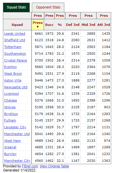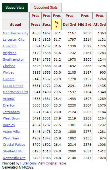We can gain deeper insight by plotting the data and computing summary statistics, as below. From the scatterplot, we can make the following qualitative statements:

There is a weak relationship between the number of pressure events and the percentage of successful pressures for each team. This could be because each team has an intrinsic efficiency at pressure events which is independent of the number of events they produce, and instead depdends on their ability and style of play. In brief: just because a team produces more pressure events, it does not mean that it also produces successful ones.
There could be a slightly inverse relationship between pressure events and success rate. A possible reason is that teams with a high number of events could be playing a more defensive style where the pressure is applied closer to their own half of the field. In these cases pressure events prioritize containment of the opponent over winning possession. Furthermore, teams that play more defensively tend to cede ball possession to the opponent. These two factors increase the opportunities of applying pressure but the intrinsic efficiency of the team remains the same, thus overall the success rate is slightly lower.
At the low end of the number of pressures: Manchester City, Arsenal, and Burnley produced very similar pressure, but Manchester City stands out as having 3.5% higher success
At the low end of success rate: Newcastle United and Sheffield United have very similar succeess rates, but Sheffield produced 700 more pressures, while Necastle;s pressure events are near the overall average of 5372
Leeds United stands out as an outlier for number of pressures, 6661, while their success rate of 29.6% is very close the the avearge of 28.9%.

Code

title = 'Percent of successful pressure events vs. total pressure events'
ylabel = 'Percent of successful pressure events'
xlabel = 'Total number of pressure events'
plot_squads(all_data,x='Press', y='%',title=title, xlabel=xlabel, ylabel=ylabel)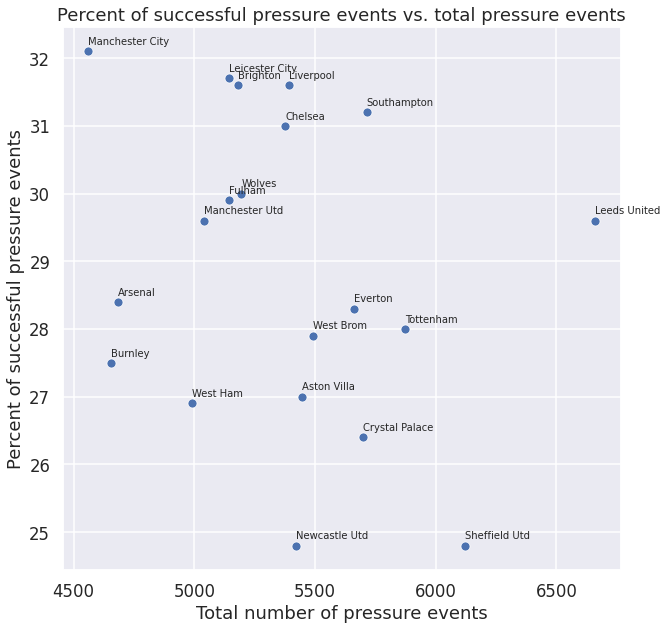

Code

all_data.describe()

	Press	Succ	%	Def 3rd	Mid 3rd	Att 3rd	Def 3rd %	Mid 3rd %	Att 3rd %	GA	GA90	SoTA	Points
count	20.00000	20.000000	20.000000	20.000000	20.000000	20.000000	20.000000	20.000000	20.000000	20.000000	20.000000	20.000000	20.000000
mean	5372.45000	1550.800000	28.915000	1852.750000	2290.850000	1228.850000	34.325000	42.645000	23.040000	51.200000	1.348000	155.100000	52.850000
std	506.83969	165.806355	2.264201	339.620357	228.299497	189.164444	4.480704	1.113305	4.012795	11.251199	0.296019	34.857454	16.887476
min	4560.00000	1282.000000	24.800000	1167.000000	1897.000000	903.000000	24.800000	40.500000	17.400000	32.000000	0.840000	89.000000	23.000000
25%	5116.75000	1470.250000	27.375000	1653.250000	2162.250000	1097.000000	31.875000	41.800000	19.950000	44.750000	1.175000	134.750000	42.500000
50%	5385.00000	1534.000000	29.000000	1885.000000	2257.500000	1256.000000	34.600000	42.850000	22.550000	49.000000	1.290000	151.000000	57.000000
75%	5670.00000	1639.250000	31.050000	2120.250000	2380.500000	1307.000000	37.925000	43.400000	25.225000	56.750000	1.495000	177.500000	65.250000
max	6661.00000	1972.000000	32.100000	2341.000000	2885.000000	1726.000000	40.600000	44.500000	32.000000	76.000000	2.000000	235.000000	86.000000

Code

fig, (ax1, ax2) = plt.subplots(1,2, sharey=True, figsize=(20,10))
subplot_squads(all_data, x='%', y='Points', ylabel='Points', xlabel='Percent of successful pressure events', ax=ax1)
subplot_squads(all_data, x='Press', y='Points', xlabel='Total number of pressure events', ax=ax2)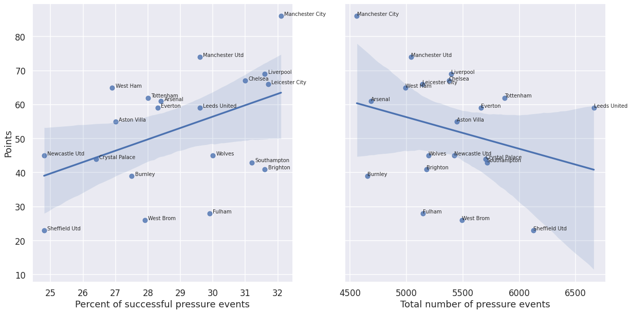

Code

points_press_corr = all_data['Points'].corr(all_data['Press'])
points_success_corr = all_data['Points'].corr(all_data['%'])

print('Correlation between points and number of pressures: {:f}'.format(points_press_corr))
print('Correlation between points and success rate of pressures: {:f}'.format(points_success_corr))

Correlation between points and number of pressures: -0.279062
Correlation between points and success rate of pressures: 0.448378

Pressure events by field location

To understand better the pressure characteristics of the teams, we can look at where the teams apply pressure: in their defensive third, middle third, or attacking third (high-press) of the pitch. The table below shows the teams ordered by the number of pressure events in the attacking third. We see that: * Liverpool produce the most pressures in the attacking third, a difference in rank of +9 compared to their total pressure events. * Leeds United and Sheffield United are 2nd and 3rd in most pressures in the attacking third, which is consistent with the fact that these two teams produce the most overall pressure events. * Manchester City are in 4th place, a difference in rank of +16 compared to their total pressure events.

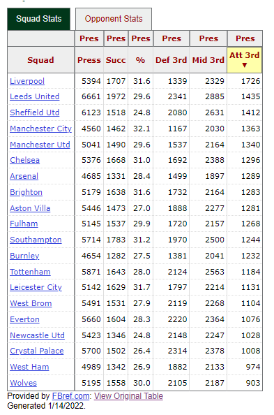
We see that Sheffield and Leeds were among the leaders for pressure events applied in the attacking third, but their final placement in the table is quite different, with Sheffield finishing last, and Leeds in 9th place. Manchester City won the championsip, but had less pressure events overall and in the attacking third than these two teams. The explanation is that we need to look at the distribution of a team’s pressure events in the three parts of the pitch, not just at the raw total counts. This gives us a picture of a team’s preferred zone of pressure application throughout the match. Thus we look at the normalized profile of the pressure events for each team, not just the raw counts. The following figure shows that there is a stonger correlation between points won and the percentage of pressure in attacking third (0.38), compared to considering the just raw numbers (0.23).

Based on these considerations, and the ones from the previous section, we understand that a team’s performance during the season depends on the relative location of their pressure activity and on the quality (success rate) of their efforts.

Code

fig, (ax1, ax2) = plt.subplots(1,2, sharey=True, figsize=(20,10))
subplot_squads(all_data, x='Att 3rd', y='Points', ylabel='Points', xlabel='Number of pressures in attacking third', ax=ax1)
subplot_squads(all_data, x='Att 3rd %', y='Points', xlabel='Percent of pressures in attacking third', ax=ax2)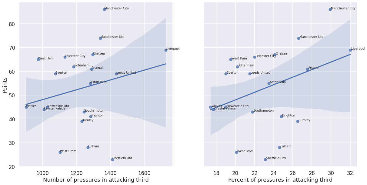

Code

points_att_pct_corr = all_data['Points'].corr(all_data['Att 3rd %'])
points_att_num_corr = all_data['Points'].corr(all_data['Att 3rd'])

print('Correlation between points and number of pressures in the attacking third: {:f}'.format(points_att_num_corr))
print('Correlation between points and percent of pressure in the attacking third: {:f}'.format(points_att_pct_corr))

Correlation between points and number of pressures in the attacking third: 0.231986
Correlation between points and percent of pressure in the attacking third: 0.378874

Relationship to goals-against (GA) and shots-on-target-against (SoTA)

In the previous sections we looked at the relationship between a team’s defensive pressure characteristics, which we narrowed to pressure success rate and proportion of pressure in the attacking third, and the points earned by the team. We now do the same for the GA and SoTA team metrics. To begin with, let’s look at the FBref statistics are in the table below:

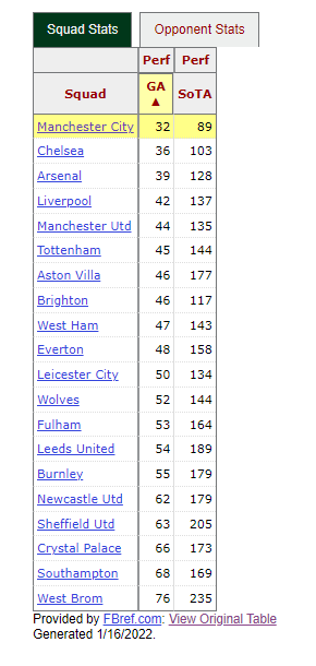
Observations:

Manchester City has the fewest GA (32) and by far the fewset SoTA (168).
Sheffield United have the 4th highest GA (53) and the scond-highest SoTA (205)

Relating these statistics with the previous section we, see that the team with be best GA and SoTA preformance (Man City) produced the fewest pressure events, but also had the highest success rate and one of the highest proportions of pressures in the attacking third. Conversely, Sheffield United produced the most pressure events, but with low success and more of the events in its own third. while also having some of the worst GA and SoTA metrics. Therefore, it is not the raw number of pressures that makes a difference, but how the pressure is applied: the success rate and, to a lesser but still significant degree, the location of the pressure.

Indeed the plots below and the corresponding correlation coefficients show a strong negative correlation between GA and SoTA and the success rate and the location of the pressure events:

	Pressure success %	Attcking third pressure %
GA	-.56	-.47
SoTA	-.44	-.63

GA and SoTA are more closely related to the pressure characteristics than points, because they measure quantities more directly dependent on how the team plays: they are closer to the dynamics of the game. The above results also make intuitive sense: the higher the team’s pressure, the less opportunities the opponent will have to take shots on goal, because the opponent is forced to expend effort in their own half and work around the press, away from the team’s goal. On the other hand, while effective at reducing SoTA, a high press may not necessarily result in winning possession, so the success rate becomes more important as it relates to GA.

These results, together witht he comments made in the prevous section, explain the difference in performance between Manchester City and Sheffield United.

Code

fig, (ax1, ax2) = plt.subplots(1,2, sharey=True, figsize=(20,10))
subplot_squads(all_data, x='%', y='GA', ylabel='GA', xlabel='Percent of successful pressures', ax=ax1)
subplot_squads(all_data, x='Att 3rd %', y='GA', xlabel='Percent of pressures in attacking third', ax=ax2)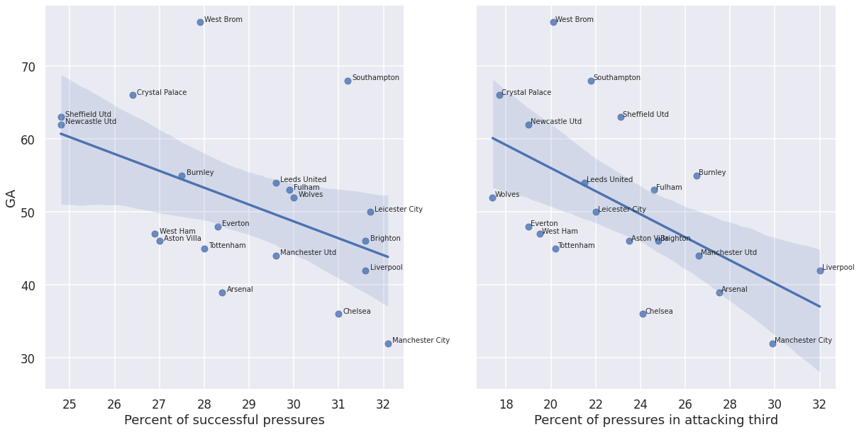

Code

ga_att_pct_corr = all_data['GA'].corr(all_data['Att 3rd %'])
ga_suc_pct_corr = all_data['GA'].corr(all_data['%'])

print('Correlation between GA and success rate of pressures: {:f}'.format(ga_att_pct_corr))
print('Correlation between GA and percent of pressure in the attacking third: {:f}'.format(ga_suc_pct_corr))

Correlation between GA and success rate of pressures: -0.563937
Correlation between GA and percent of pressure in the attacking third: -0.465390

Code

fig, (ax1, ax2) = plt.subplots(1,2, sharey=True, figsize=(20,10))
subplot_squads(all_data, x='%', y='SoTA', ylabel='SoTA', xlabel='Percent of successful pressures', ax=ax1)
subplot_squads(all_data, x='Att 3rd %', y='SoTA', xlabel='Percent of pressures in attacking third', ax=ax2)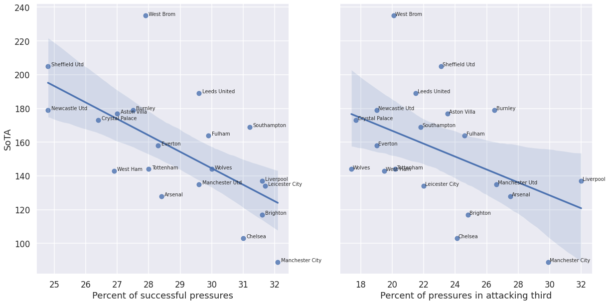

Code

sota_att_pct_corr = all_data['SoTA'].corr(all_data['Att 3rd %'])
sota_suc_pct_corr = all_data['SoTA'].corr(all_data['%'])

print('Correlation between SoTA and success rate of pressures: {:f}'.format(sota_att_pct_corr))
print('Correlation between SoTA and percent of pressure in the attacking third: {:f}'.format(sota_suc_pct_corr))

Correlation between SoTA and success rate of pressures: -0.440233
Correlation between SoTA and percent of pressure in the attacking third: -0.633339

Discussion

I repeat here the summary from the introduction, and conclude with a paragraph on choosing the right metrics.

Finally, it is important to distinguish overall win/lose-type of statistics, from more descriptive statistics. While a team’s overall objective is to win, the objective of a tactical/match analyst is to understand their own team and the opponents: simple winning statistics are not as helpful here. Instead, choosing metrics more closely connected to the actions taken on the field, like GA and SoTA in this case, yields deeper undertanding and more fruitful exchange of ideas.

License You may use and modify this Jupyter notebook under the terms of the BSD license.