Exploring soccer heatmaps from Tracab XML files with tfutils.py
tfutils.py is a Python library for reading and interacting with soccer data from Tracab XML files.
soccer analytics
python
tracab
heatmap
xml
Author
Luca Cazzanti
Published
November 20, 2022
Summary
A Tracab TF05 feed is an XML file that contains data about a soccer match. In particular, a TF05 feed provides various flavors of heatmaps of the two teams and of the individual players who took part in the match. In this note I describe the structure of the of a Tracab TF05 XML file and show how to use the tfutils.py Python library to easily read and plot the team and player heatmaps. tfutils not about a fancy ML algorithm that detects line-breaking passes or identifies formations from video. It is a simple tool that saves analysts time and speeds up the analysis. As a use case, I look at the TF05 XML file from the Syria vs. Mauritania match of 6 December 2021, group stage of the Arab Cup.
The background for this work is that I’ve been doing some pro-bono soccer analytics for a men’s national team participating in the FIFA World Cup in Qatar. The team receives TF05 feeds, but does not have a developed data processing infrastructure, so the work must be done manually. I grew frustrated with having to use low-level XML parsing methods every time I wanted to locate and plot the heatmap data from the file, so I wrote the tfutils Python library to save myself time. The tfutils API abstracts away the low-level XML methods, and uses soccer semantics to read and plot the data. For example, you can use intuitive method calls like data.team_heatmap('home') and data.get_team_players('away'). However, low-level XML parsing methods are retained, giving data analysts a choice of interfaces to the TF05 feed. I hope that the following write-up conveys how soccer analysts can get off the ground quickly with coarse but meaningful analyses based on TF05 hetamaps with just a few lines of Python code. These analyses can be a component of more comprehensive pre- or post-match analyses.
Content and structure of a Tracab TF05 XML file
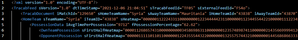
Tracab TF05 XML files contain summary match data, like team names, player names, match date, but the heatmaps make up bulk of the information. These heatmaps summarize the pitch locations where teams and individual players have been present. This information can form part of pre- and post-match analysis reports, or general opponent research. The first few lines of a Tracab TF05 XML file look like this:
THere are two families of heatmaps: combined team heatmaps and infividual player heatmaps.
Combined team heatmaps
Overall: combined team heatmap, over the entire match duration
Defence: combined heatmap of the team defenders
Midfield: combined ehatmap of the team midfielders
Attack: combined heatmap of the team attackers.
Unfortunately, the Tracab TF05 feed does not tell us which players are part of the defence, midfield, and attack heatmaps, so we are left with just an intuitive notion of which players contribute to which heatmap and we’d have to cross-reference with other sources of information. Nonetheless, let’s assume Tracab have done a good job categorizing the players into the apprpopriate hetamaps. On the positive side, we have access to team heatmaps separated by phases of the game (in/out of possession) and by period (first half, second half):
In possession or out of possession. For each of these two phases, we have these combined team heatmaps:
Overall
First half
Second half
Individual player heatmaps
Similar to the combined team heatmaps, possession heatmaps are available for each player, in addition to the player’s overall heatmap. First-half and second-half heatmaps are not available for individual players.
Overall: a player’s overall heatmap for the entire match duration.
In possession or out of possession. For each of these two phases, we have these player heatmaps:
Overall
First half
Second half
Structure of a heatmap
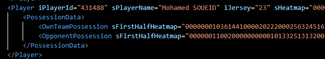
A heatmap in a Tracab TF05 feed is represented as a long string of 240 character digits, each digit an integer between 0-9. These 240 digits are associated with 240 pitch locations, and represent the time a team (or a player) spent in that location. The numbers 0-9 are normalized time values, where 0 means “no time” and 9 means “most time.” Unfortunately, I do not know the normalization applied to the time spent in each location, so I cannot say what “most time” means. For this reason, I take the safe approach to interpreting these numbers and view them only relative to the rest of the same heatmap, and not relative to other heatmaps. So for example, I cannot tell if a “9” from player X represents the same absolute length of time as a “9” for player Y, but I am sure that for player X a “9” means more time spent in a particular location than a “4” for the same player. Here’s what a heatmap tag looks like in the XML feed:
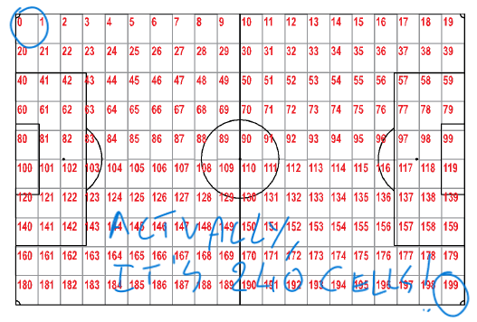
The 240 character digits map to a 24x20 matrix overlaid on the pitch, with the top left corner corrsponding to the first digit, and the bottom right corner to the last. Here’s a snapshot from Tracab’s documentation, which however is incorrect! The documentation states that heatmaps are made of 200 digits (20x10), but I found out the hard way while writing tfutils that it’s actullally 240. Nonetheless, the figure below gives you the general idea. Note that all heatmaps assume that the attacking direction is left-to-right, irrespective of the actual attacking direction during the match. In other words, all heatmaps have been standardized on a left-to-right attacking reference for the entire match and for the halves.
Plotting the team-level heatmaps
Getting started with TF05 file, you’ll want to read basic information about the match, get a list of players, and plot the two team’s heatmaps. It’s interesting that this XML feed does not include the final score. I guess a club that uses Tracab as data provider would have access to other Tracab feeds, which merged with this one, give a more complete picture of the match, including the final score. In any case, I happen to know that the final score for this match was Syria 1 - Mauritania 2.
from tfutils import TracabTf05Xmlsource = TracabTf05Xml('/home/luca/projects/tfutils/data/129650_TF05_PMS.xml')source.parse()source.summary()
Source file: /home/luca/projects/tfutils/data/129650_TF05_PMS.xml
Home team name and ID:Syria, 43838
Away team name and ID: Mauritania, 43870
Match date: 2021-12-06 18:00:00
Match ID: 129650
Match duration: 98.614 minutes
Syria and Mauritania’s overall heatmaps
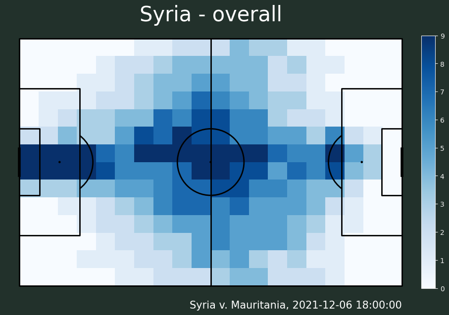
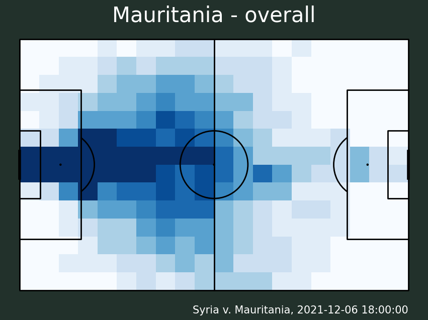
Let’s start simple: the overall heatmaps for the two teams. Immediately we can see that Syria, the home team, explored more of the length of the pitch, especially the central channel. Mauritania, instead, spent more time in its own half. So, chances are that Syria attacked more and had more ball possession that Mauritania, which likely was either content to apply a low block, or was pressured by Syria into a more defensive stance. These are preliminary hypotheses for sure but what I like about this approach is that you can immediately start formulating ideas about what happened during the match which can guide your subsequent analysis steps. Of course you should cross-check with other sources of information, including actually watching the match of course!
p = source.team_heatmap('home', add_cbar=True)# You can also call this method with the name of the team# source.team_heatmap('Syria')
p = source.team_heatmap('away')
Heatmaps for defense, midfield, and attack
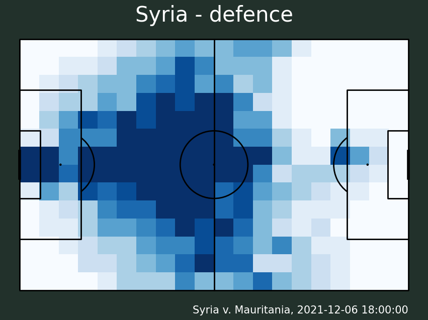
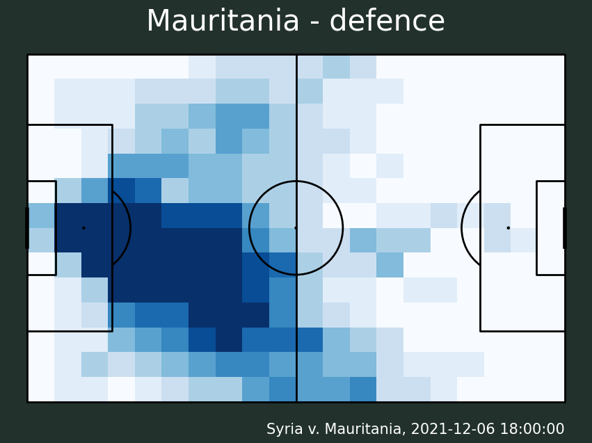
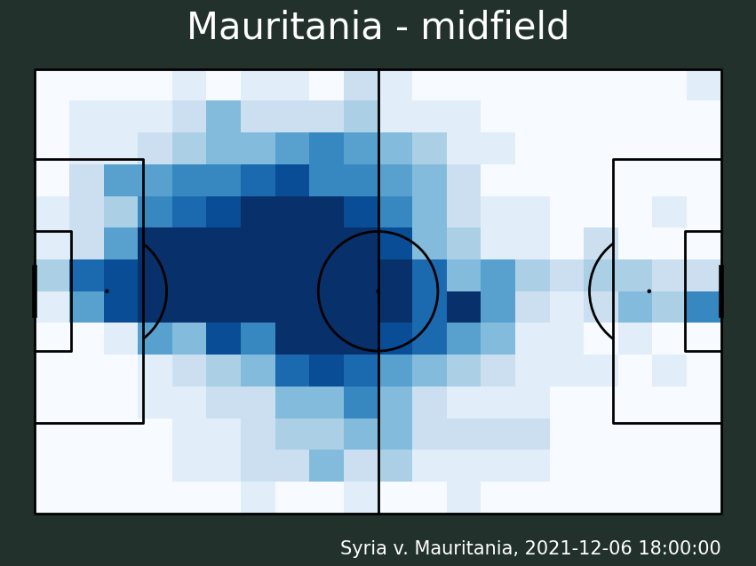
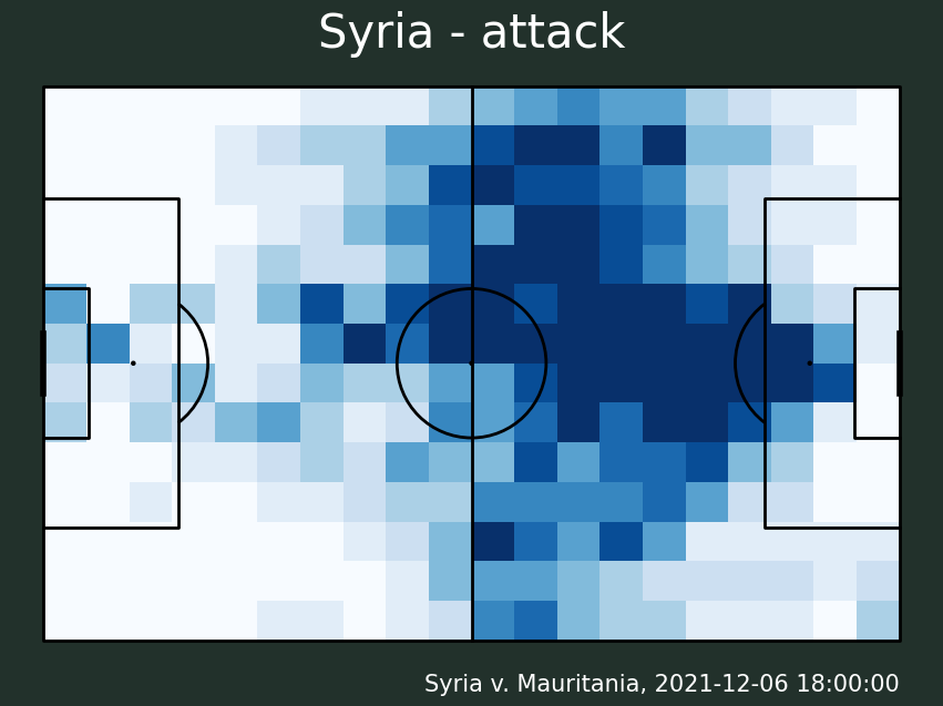
It is not surprising that when breaking down the heatmaps of the two teams by unit, we see patterns consistent with the overall heatmaps above. Syria pushed into Mauritania’s half more, mostly in the central channel, while Mauritania swelled more in its own half; in fact Mauritania’s attackers seem to have spent more time close to the midfield, while the midfielders were essentially playing defense. One thing stood out to me when comparing Syria’s defense with Maritania’s. In Syria’s case, the defenders cover both the right and left sides in a symmetrical cone, following almost exactly the shape of the defensive funnel. In contrast, Mauritania’s defenders covered the right (bottom) half od the funnel, while the midfielders covered the left (top). However, remember that we do not know how Tracab decides which players are defenders and which ones are midfielders, so it is possible that this is an artifact of the data rather than an actual tactical choice by Mauritania. This is where other sources of information, like video form the match, other data feeds, or tour colleagues in the club’s tactics team can help get a deeper understanding.
p = source.team_heatmap('Syria', hm_type='defence')p = source.team_heatmap('Mauritania', hm_type='defence')
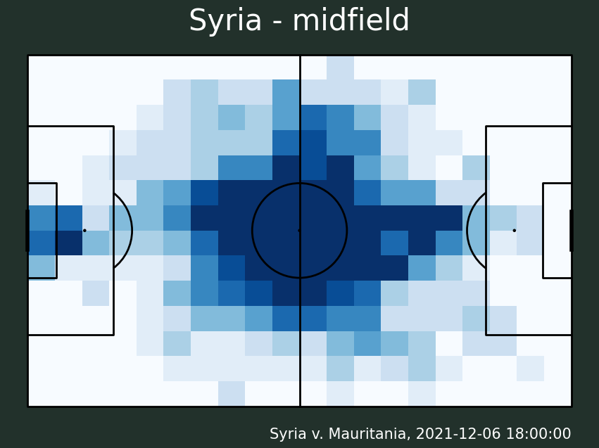
p = source.team_heatmap('Syria', hm_type='midfield')p = source.team_heatmap('Mauritania', hm_type='midfield')
p = source.team_heatmap('Syria', hm_type='attack')p = source.team_heatmap('Mauritania', hm_type='attack')
Heatmaps by possession phase
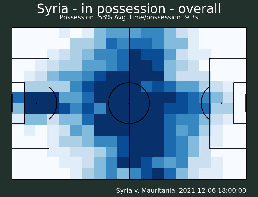
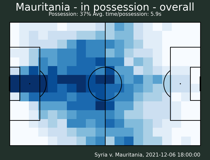
Looking at the heatmaps of the two teams while they are in possession, again we see that Syria’s center of mass is shifted toward the opponent’s half, while Mauritania dwells in its own half. So perhaps Mauritania had trouble getting out of its half, or maybe thay had a deliberate strategy to play long balls into the attack, which typically result in lower time of possession in the attacking third. The possession statistics from the TF05 file are aligned with this line of thinking, too: Syria had 63% possession and its possession sequences where 39% longer than Mauritania’s (9.7 seconds vs. 5.9 seconds). Again, watching the video will help clarify these hypoteses, but isn’t it cool that we can get a general idea of how the teams played from just a few summary heatmaps?
p = source.team_possession_heatmap('Syria', possession='in')p = source.team_possession_heatmap('Mauritania', possession='in')
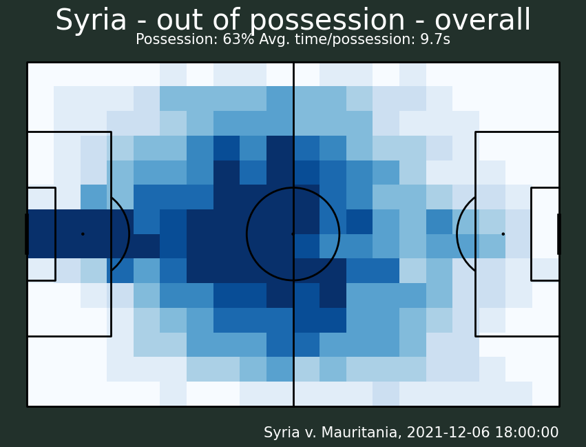
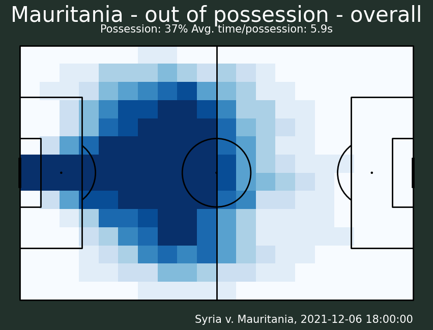
Inspecting the heatmaps when the teams are out of possession, we see that Syria’s block is a bit higher up the pitch than Mauritania’s. consistent with previous observations. Note how Mauritania’s heatmap is an almost perfect defensive funnel. Visually, it’s as if the defence and midfield heatmaps from the above discussion were combined into one to obtain the out-of-possession heatmap. This hints again at Mauritania employing their midfield mostly in a defensive stance, supporting the defensive unit.
p = source.team_possession_heatmap('Syria', possession='out')p = source.team_possession_heatmap('Mauritania', possession='out')
Plotting the heatmaps of individual players
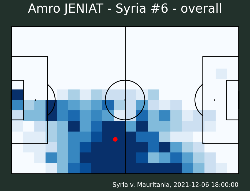
You can easily get to overall and possession heatmaps for individual players. The overall heatmap also includes the player’s overall average position as a red dot. Here’s the example of a right midfielder on Syria.
p = source.player_heatmap('Amro JENIAT')
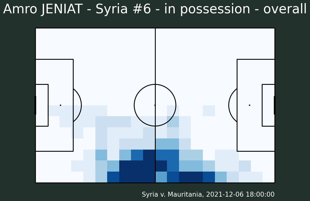
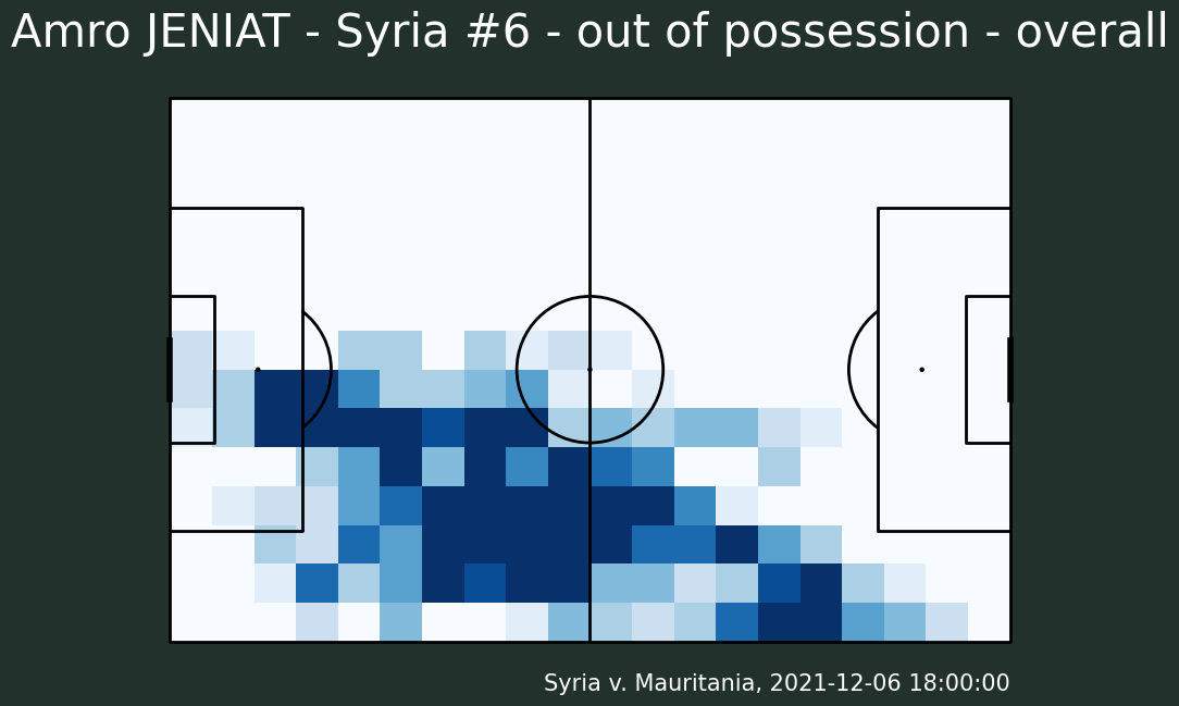
The possession heatmaps, similar to the team-level heatmaps, tell us a player’s positioning while the player’s team is in or out of possession. In the example below we see that the same Syrian right midfielder, Amro Jeniat, pinches in toward the center when Syria is out of possession, which is a resonable behavior when you are containing the opponent and applying pressure in the middle third. However we also notice that he visits the right-most edge of the attacking third while out of possession. Possibly, he is applying high pressure on Mauritania’s left defender or midfielder while Mauritania is building up.
p = source.player_possession_heatmap('Amro JENIAT', possession='in')p = source.player_possession_heatmap('Amro JENIAT', possession='out')
Discussion
Soccer clubs that are farther along in their data maturity have robust data engineering practices, comprising automated ingestion pipelines that take external data feeds (including XML Tracab files) and put them in databases. These databases in turn power downstream visualizations and drill-down analyses. However, many clubs are merely getting started with data and do not have any of the processes in place. If you are working for one of these less data-mature clubs then tfutils will help you get started with your analyses by providing intuitive interfaces to the XML TF05 feed.
I showed how being able to easily inspect the heatmaps in the TF05 files lets us formulate hypotheses about how the two teams and the individual players behaved during a match, which can make further analyses more efficient. Similarly, analysts may who have viewed the video from a match may be interested in producing quick visualizations of a player’s locations on the pitch to corroborate or disrpove their observations with data, or to create match reports for the technical staff. Either way, tfutils helps with easy access to the underlying data in the Tracab TF05 XML files. Installation instructions and a README are on GitHub.
> git clone git@github.com:your_fork/tfutils.git> cd tfutils> pip install-r requirements.txt .# ... or, to install the dev version:> pip install-r requirements.txt -e .# If you prefer make:> make install# ... or ...> make dev-install
Main features
Currently tfutils cosists of class TracabTf05Xml which inherits from class xml.etree.ElementTree.ElementTree. So you can use the lower-level XML parsing methods of ElementTree in addition to the soccer-specific methods of TracabTf05Xml. For example, the following are two equivalent ways to get a player’s data from the XML file:
# using XML doc parsing (this is what happens inside the get_player() method)home_team = source.find('HomeTeam')player ="Megan RAPINOE"query ="Player/[@iPlayerId='{}']".format(player)team = source.find('HomeTeam')player_node = team.find(query)# ...using soccer semantics:player ="Megan RAPINOE"source.get_player(player)
The heatmap methods accept keyword arguments for customizing the plots.
pitch_kwargs: any keyword arguments that can be provided to mplsoccer.Pitch().
hm_kwargs: any keyword arguments that can be provided to pitch.heatmap().
grid_kwargs: any keyword arguments that can be provided to pitch.grid().
TracabTf05Xml() uses reasonable defaults for colors, fonts, figure size if no keyword arguments are provided. Here the definition of “reasonable” is “it works sufficiently well for my purposes.” I did the best I could to ensure the defaults work well together, and they do, but there’s room for improvement, and some paramters are still hard-coded. You can inspect the default plotting parameters as follows:
You can inspect additional XML document properties through corresponding object properties. The __init__ method of TracabTf05Xml sets the properties to None and the parse() method assigns them the corresponding values from the XML file (which could be empty strings). The summary() method prints the main properties. See the [README on GitHub]((https://github.com/lucacazzanti/tfutils) for a full list of object properties.
source.summary()
Source file: /home/luca/projects/tfutils/data/129650_TF05_PMS.xml
Home team name and ID:Syria, 43838
Away team name and ID: Mauritania, 43870
Match date: 2021-12-06 18:00:00
Match ID: 129650
Match duration: 98.614 minutes
Future work
At the moment tfutils supports only TF05 files, but can easily be expanded to other Tracab XML files, and possibly other Tracab, non-XML feeds. The wonderful library Kloppy already provides an interface for reading Tracab .dat tracking data files into a pandas dataframe, so one possibility could be to expand tfutils with methods for merging that data with the XML files to provide a comprehensive view of a soccer match.